Classification
Learning Objectives
- Understand the difference between supervised and unsupervised learning
- Implement and explain basic classification (e.g., decision trees) and clustering (e.g., K-means) algorithms
- Use real-world traffic incident data to solve classification and clustering problems
- Interpret model outputs and performance metrics
Definition: Classification is the task of predicting a label or category for input data. In our case, we might classify an incident based on its description as a "Crash", "Traffic Hazard", or "Loose Livestock".
Real-Life Analogies
- Spam filter: Given the contents of an email, predict whether it's "Spam" or "Not Spam".
- Doctor's diagnosis: Based on symptoms, classify a disease.
- Campus security: Given an incident report, predict if it's high priority.
Algorithm Focus: Decision Trees
How It Works
- A decision tree splits the data based on the features to reduce uncertainty.
- Each split is a "yes/no" question (e.g., Does the incident description contain 'crash'?)
- It continues splitting until it can confidently assign a label.
Intuitive Explanation
Think of playing 20 Questions, where you narrow down the object by asking binary questions. A decision tree is doing exactly that—asking a series of smart questions to guess the right label.
Math Behind It
- Entropy (information gain): measures uncertainty. Lower entropy \= more confidence.
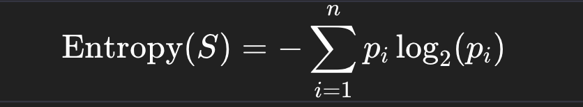
Entropy formula from Information Theory, which is also used inside Decision Trees (like ID3, C4.5, CART) to decide where to split the data.
What it means:
- S = a dataset (or subset) at a node in the tree.
- n = the number of possible classes (e.g., "Highway" vs "Local" → 2 classes).
- pi = the proportion (probability) of examples in class i within dataset S.
- log₂ = base-2 logarithm, which measures information in "bits."
Intuition
- Entropy measures uncertainty or impurity in the dataset.
- If all samples belong to a single class then entropy = 0 (pure, no uncertainty).
- If samples are evenly split between classes then entropy is maximum (most uncertain).
Example with Highway vs Local:
Say at some node:
- 8 incidents are Highway
- 2 incidents are Local
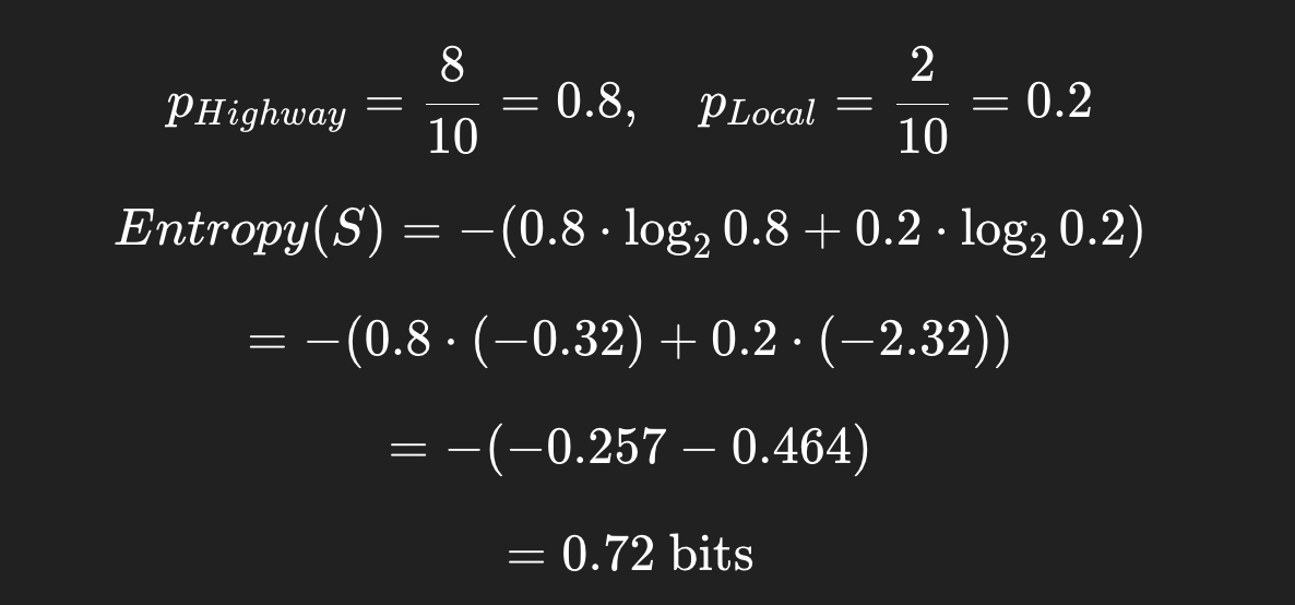
So this node has some uncertainty (not perfectly pure), but leaning strongly toward "Highway."
Information Gain:
Step 1: Entropy
If a node is perfectly pure (all "Highway"), entropy = 0.
If it's a 50/50 split (max uncertainty), entropy = 1 (for binary classification).
Step 2: Splitting the Data
Suppose we're trying to classify Highway vs Local. We pick a feature (say, "Street Name starts with 'I-' → interstate). Splitting on this feature divides the dataset into subsets.
- Subset A: incidents where
Street starts with I- - Subset B: incidents where
Street does not start with I-
Each subset will have its own entropy.
Step 3: Weighted Average Entropy After Split
After the split, the expected entropy is:

- The algorithm chooses the feature/split that maximizes information gain.
- Sj = subset j
- ∣Sj∣/∣S∣ \= proportion of samples in that subset
Step 4: Information Gain
The information gain tells us how much uncertainty was reduced:
IG(S,feature)=Entropy(S)−Entropysplit
- If IG is high, that feature is a great split (makes subsets purer).
- If IG is low, the feature doesn't help much.
Example with Numbers
Say we have 10 traffic reports:
- 6 Highway, 4 Local
Entropy before split:
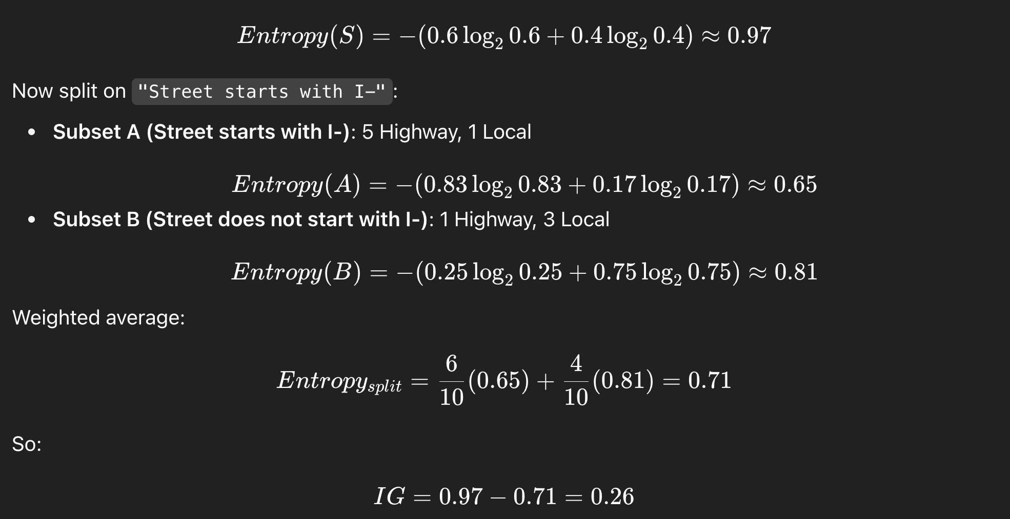
Interpretation:
Splitting on "Street starts with I-" reduces uncertainty (good feature). The decision tree will prefer this feature if no other feature has higher information gain.
Classification Lecture: Highway vs Local
Learning Objectives
By the end of this lesson, students will:
- Understand the difference between simple queries, logistic regression, and decision trees for classification.
- Be able to classify incidents as Highway vs Local using
locationoraddress. - Visualize and interpret a Decision Tree.
- Critically think about feature engineering and model limitations.
Simple Query / Filtering Approach
Concept: Use keywords to classify incidents without ML.
This works because location/address contains highway identifiers.
import pandas as pd

# Load dataset
df = pd.read_csv("austin_traffic_incidents.csv")

# Highway keywords
highway_keywords = ["I-35", "IH-35, "US 183", "Mopac", "Loop 1", "SH 71"]

# Classify using simple filter
df['road_type'] = df['address'].fillna("").str.upper().apply(
    lambda x: "Highway" if any(k.upper() in x for k in highway_keywords) else "Local"
)

print(df['road_type'].value_counts())
Teaching Notes / Analogy:
Think of this like a "keyword detector", a quick rule-of-thumb classifier.
Student Challenge:
-
Modify the code to include more highway identifiers.
-
Count how many incidents are classified differently if you add/remove keywords.
Logistic Regression in a nutshell
The Problem
- Linear Regression predicts continuous values (like predicting temperature or house price).
- But sometimes we want to predict categories (e.g., “Highway” vs “Local” or “Accident” vs “Non-Accident”).
The Trick
- Logistic Regression takes a linear combination of inputs (like Linear Regression does), but instead of outputting any number on the real line, it squashes it into a range between 0 and 1 using the sigmoid function:

The Output
The output is interpreted as a probability:
- If P(y=1|x)>0.5 → predict class 1 (e.g., Highway).
- If P(y=1|x)<=0.5 → predict class 0 (e.g., Local).
Why It's Useful
- Logistic Regression is one of the simplest, most interpretable classification algorithms.
-
It's often a baseline model before trying more complex ones (like Decision Trees, Random Forests, or Neural Nets).
-
It gives you probabilities, not just a hard class label, which can be very valuable.
In the Austin Traffic dataset example:
We could use Logistic Regression to classify whether an incident is on a Highway (1) or Local road (0) based on features like latitude, longitude, issue_reported, etc.
Logistic Regression Baseline
Concept: Use address text and/or issue_reported as features.
- Convert text to numeric with
CountVectorizerorTfidfVectorizer.
Side quest: CountVectorizer
- Turns text into numbers by counting words.
- It builds a vocabulary of all unique words across your dataset.
- Each text entry (like an incident description) becomes a vector where each dimension is the count of a word in that entry.
Example: Suppose we have three reports:
-
"Crash on highway"
-
"Stalled vehicle"
-
"Crash on local road"
Vocabulary = [crash, on, highway, stalled, vehicle, local, road]
Vectors:
-
"Crash on highway" →
[1,1,1,0,0,0,0] -
"Stalled vehicle" →
[0,0,0,1,1,0,0] -
"Crash on local road" →
[1,1,0,0,0,1,1]
TfidfVectorizer (Term Frequency–Inverse Document Frequency)
- Similar to
CountVectorizer, but instead of raw counts, it weighs words by how important they are. - Common words like "on" or "road" appear in many reports → less informative → down-weighted.
- Rare but meaningful words like "fatality" or "hazmat" get higher weight.
- Logistic Regression predicts probability of Highway vs Local.
from sklearn.model_selection import train_test_split
from sklearn.feature_extraction.text import CountVectorizer
from sklearn.linear_model import LogisticRegression
from sklearn.metrics import classification_report

# Features and labels
X = df['address'].fillna("")
y = (df['road_type'] == "Highway").astype(int)

# Text to numeric features
vectorizer = CountVectorizer()
X_vec = vectorizer.fit_transform(X)

# Train/test split
X_train, X_test, y_train, y_test = train_test_split(X_vec, y, test_size=0.2, random_state=42)

# Train Logistic Regression
clf = LogisticRegression(max_iter=200)
clf.fit(X_train, y_train)

# Evaluate
y_pred = clf.predict(X_test)
print(classification_report(y_test, y_pred))
Teaching Notes / Analogy:
Logistic Regression is like drawing a smooth boundary between Local and Highway based on text features.
Student Challenge:
- Try using
issue_reportedinstead ofaddress. - Compare performance: which feature gives better classification?
Decision Tree Approach
Concept: Visual, interpretable classification.
The tree splits on features like keywords in address.
from sklearn.tree import DecisionTreeClassifier, plot_tree`
import matplotlib.pyplot as plt

# Train Decision Tree
tree = DecisionTreeClassifier(max_depth=4, random_state=42)
tree.fit(X_train, y_train)

# Evaluate
print("Accuracy:", tree.score(X_test, y_test))

# Visualize the tree
plt.figure(figsize=(16,10))
plot_tree(tree, feature_names=vectorizer.get_feature_names_out(),
          class_names=["Local", "Highway"], filled=True, fontsize=10)
plt.show()
Teaching Notes / Analogy:
The Decision Tree is like a flowchart: each node asks a question (“Does the address contain I-35?”) and routes the incident down the appropriate branch.
Student Challenge:
- Change
max_depthand see how the tree grows/shrinks. - Identify which words/features the tree uses to split.
- Compare Decision Tree vs Logistic Regression performance.
Wrap-Up Discussion Prompts
- Why might a simple query work well for Highway vs Local? When might it fail?
- What advantages does ML provide over keyword rules?
- How could you add additional features (time, lat/lon, issue_reported) to improve classification?
- How would you evaluate whether Logistic Regression or Decision Tree is “better”?
- Could you extend this to multi-class classification (e.g., different highway types or traffic incident types)?
Optional Extensions / Challenges
- Predict peak vs off-peak highway usage using time features.
- Combine Decision Tree with latitude/longitude clustering to see patterns on a map.
- Try Random Forest to see if ensemble methods improve accuracy.